In the world of data science, logistic regression is an essential tool for predicting outcomes based on given input variables. The primary goal of this blog is to provide a detailed explanation of logistic regression and its usefulness, along with an introduction to the ROC Curve, its interpretation, and how to use it to validate logistic regression models.

What is Logistic Regression?

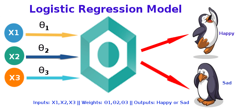
Logistic regression is a statistical method that is used to analyze the relationship between a dependent variable (often binary) and one or more independent variables. It is particularly useful in scenarios where the response variable is dichotomous, that is, it can take either of the two possible outcomes. For example, whether a patient has a disease or not, whether a customer will buy a product or not, whether a student will pass or fail, and so on.

The outcome variable in logistic regression is usually modeled using a logistic or sigmoid function. This function maps any real-valued input to a value between 0 and 1, which can be interpreted as the probability of the binary outcome. The logistic regression model estimates the parameters of the function, which can then be used to predict the outcome of new observations.

Logistic regression can handle both categorical and continuous predictor variables, and it is relatively easy to interpret compared to other complex algorithm models.

ROC Curve

The ROC curve is a plot of the true positive rate (TPR) against the false positive rate (FPR) for different thresholds of a binary classifier. In a logistic regression model, the output is a probability value that represents the likelihood of a data point belonging to the positive class. By default, this threshold is set to 0.5, which means that any data point with a probability greater than 0.5 is classified as positive, and any data point with a probability less than 0.5 is classified as negative.

To create the ROC curve, you need to vary this threshold value and calculate the TPR and FPR for each threshold. The TPR is the proportion of true positives (i.e., positive samples that are correctly classified as positive) out of all positive samples, while the FPR is the proportion of false positives (i.e., negative samples that are incorrectly classified as positive) out of all negative samples. By varying the threshold, you can generate a set of (TPR, FPR) pairs that represent the performance of the classifier at different levels of sensitivity and specificity.

Once you have calculated the TPR and FPR for each threshold, you can plot them on a graph to create the ROC curve. The ROC curve is a plot of the TPR against the FPR, where each point on the curve represents a different threshold value. The ideal classifier would have a TPR of 1 and an FPR of 0, which means that it correctly identifies all positive samples without misclassifying any negative samples. Therefore, the closer the ROC curve is to the top-left corner, the better the performance of the classifier.

Conclusion

Logistic regression is a powerful tool for predictive modeling, especially when the outcome variable is binary. The ROC curve is a useful tool for evaluating the performance of binary classifiers and can be used to validate logistic regression models. The AUC value provides a measure of the classifier’s overall performance, while the discrimination capacity provides insights into how well the model differentiates between the two classes.

In summary, logistic regression and ROC curve analysis are essential tools in data science, and mastering them can go a long way in developing accurate predictive